Using multiple linear regression Predict the profit of startups

Predict the profit of startups by using multiple linear regression

Here is my first Blog, In this, I will mention how to develop a machine learning model to predict the profit of startups. For this model, we have some prior data with the following attributes.

=> R&D Spend Amount invested in Research and development.
=> Administration: Amount invested in administration.
=> Marketing Spend: Amount invested in marketing.
=> State: company starts from this state.

So, based on these data we will learn step by step development of Machine learning model to predict the profit. Here in this post, we will use python.

Let's Start.

Step 1: 

First, We will import some python libraries which we are going to use for our model development.

#Pandas is used for importing datasets.
#Numpy is used for mathematical functions.
#Matplotlib is a plotting library used for plotting graphs.
#Seaborn is a Python visualization library based on matplotlib.

#Warning messages are typically issued in situations where it is useful to alert the user of some condition in a program, where that condition (normally) doesn’t warrant raising an exception and terminating the program. For more info click here

Step 2 :

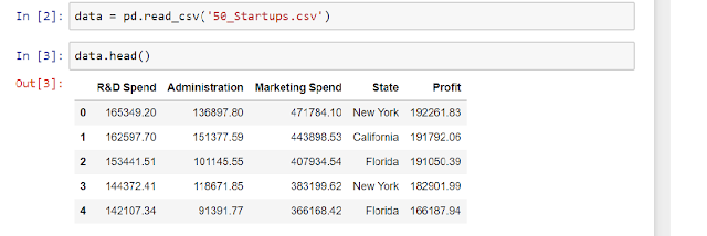
Import 50 startups datasets using the read_csv function of pandas.

Step 3 :

check the number of null value in data attributes and type of data.

We don't have any null value attribute.

Step 4 :

Let's Analyze the attributes one by one. data.head()

R&D Spend: Numerical values.

Administration: Numerical values.

Marketing Spend: Numerical values.

State: Categorical values.

we will not get any useful information by Visualizing the Numerical values.

So, we will focus on the Categorical variable "State".

Lets see the counterplot bar graph of State's categorical variable.

Here we will plot this bar graph by using the countplot function of the seaborn library.

Note: In this graph, we can observe that all three categorical values are equally distributed.

we can also visualize this in the pie chart.

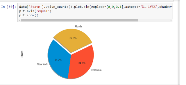
Lets plot bar graph and pie chart together in two subplots.

Step 5:

After visualization of attributes of startup dataset . Now we are going to develop our model.
Here we will separate input variable and target variables.
So, In our input variable we will keep independent variable and in target variable we will keep
dependent variable here profit is our dependent variable.

Step 6:
OK, Now we have our input variable and target variable in x and y simultaneously.
let's check the data type of x .

Now we can see the x data type is 'O' = object because of State attribute , we can't apply linear regression model on object data type , So we need to convert it into float type.

#We will use dummy variable concept to replace categorical variable.

e.g:

  New York = D1 (dummy 1) if yes : 1 else : 0

  California = D2 (dummy 2) if yes : 1 else : 0

  Florida = D3 (dummy 3) if yes : 1 else : 0

but we will go with one less number of dummy variable.

i.e.  D1 and D2 .

if D1=1 and D2=0 it is in New York

if D1=0 and D2=1 it is in California 

if both D1=0 and D2 = 0 than it is in Florida 

%%Our machine learning model is intelligent enough to understand it %%

So let's use dummy variable 

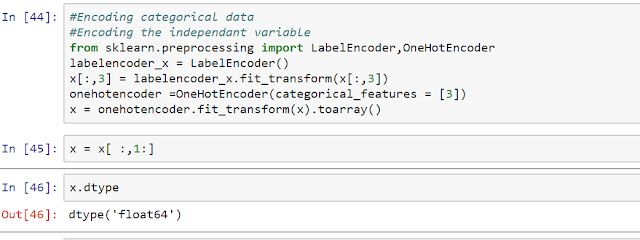
To do this, we are using LabelEncoder and OneHotEncoder from sklearn.preprocessing.

Now we can see that our input variable is float type. 

%%If you want to know more about it you can query in comment section%%

Step : 7

To develop linear model we need some amount of data to train our machine, and after training we also need to test our model.So we will divide our data into training dataset and testing dataset.

we will divide it in the ratio  80:20 .

lets do it.

we will provide more data to train our model than to test the model.

Step : 8

Finally, we are going to build our model by fitting the multiple linear regression into our training set.

Step :9 

Our model is ready.  Now,lets test it by using testing dataset.

Here y_pred is predicted profit by our newly developed multi_linear model.

=>>>Do a comparison between y_pred and y_test.

Our model is developed but is not fully optimized yet.

Step 10: 

Now I am going to apply Backward Elimination to optimize our Model.(I will explain this method in my next post)

And Here is the summary of our optimized machine learning model.

You can see P value is 0.000. It means that now our model is fully optimized for 5% significant level. (Explanation of this Optimization will be mentioned in my next post.)
Thank you.